Breadth-First Search (BFS)

1. Overview

Bread-first search is one of the simplest algorithms for searching a graph and the archetype for many important graph algorithms.

Given a graph G = (V,E) and a distinguished source vertex s, breadth-first search systematically explores the edges of G to “discover” every vertex that is reachable from s. It computes the distance from s to each reachable vertex, where the distance to a vertex v equals the samllest number of edges needed to go from s to v.

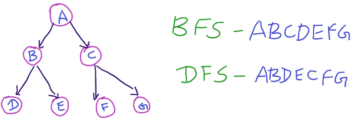
In trees, Breadth-First Search (BFS) start with the root, move left to right across the second level, then move left to right across the third level, and so forth. You continue the search until either you have examined all the nodes or you find the node you are searching for.

BFS traverses the nodes level by level. In BFS, we start at the root (or another arbitrarily selected node) and explore each neighbor before going on to any of their children. That is, we go wide (hence breadth-first search) before we go deep.

bfs_dfs

You can think of it as discovering vertices in waves emanating from the source vertex. That is, starting from s, the algorithm first discovers all neighbors of s, which have distance 1. Then it discovers all vertices with distance 2, then all vertices with distance 3, and so on, until it has discovered every vertex reachable from s.

In order to keep track of the waves of vertices, breadth-first search could maintain separate arrays or lists of the vertices at each distance from the source vertex. Instead, it uses a single first-in, first-out queue containing some vertices at a distance k, possibly followed by some vertices at distance k+1. The queue, therefore, contains portions of two consecutive waves at any time.

To keep track of progress, breadth-first search colors each vertex white, gray, or black. All vertices start out white, and vertices not reachable from the source vertex s stay white the entire time. A vertex that is reachable from s is discovered the first time it is encountered during the search, at which time it becomes gray, indicating that is now on the frontier of the search: the boundary between discovered and undiscovered vertices. The queue contains all the gray vertices. Eventually, all the edges of a gray vertex will be explored, so that all of its neighbors will be discovered. Once all of a vertex’s edges have been explored, the vertex is behind the frontier of the search, and it goes from gray to black.

2. Key Concepts

BFS is less intuitive than DFS. The main tripping point is the (false) assumption that BFS is recursive. It’s not. Instead, it uses a queue.
If you are asked to implement BFS, the key thing to remember is using a queue. The rest of the algorithm flows from this fact.
In BFS, you need to keep track of the visited nodes.
BFS conceptually is traverse a graph the same way a virus would do it. The virus starts from a starting point (or points), and it then visits its neighbors, and then its neighbors, until all the nodes are visited.

3. Applications

A minimal and clean code snippet in your preferred language (e.g., Python, C++).
Focus on readability and clarity.

4. Implementation

In BFS, node a visits each of a's neighbours before visiting any of their neighbours. You can think of this as searching level by level out from a. An iterative solution involving a queue usually works best.

void bfs(Node root)
{
    Queue queue = new Queue();
    root.marked = true;
    queue.enqueue(root);    // Add to the end of the queue

    while (!queue.isEmpty()) {
        Node r = queue.dequeue();   // Remove from the front of the queue
        print(r);
        for_each (Node n in r.adjacent) {
            if (n.marked == false) {
                n.marked = true;
                queue.enqueue(n);
            }
        }
    }
}

5. Important Techniques

Technique 1: Brief explanation (e.g., balancing for AVL Trees).
Technique 2: Description (e.g., traversal methods like Inorder, Preorder).
Techniques/Variants
Any important variations or optimizations of the algorithm (if applicable).

6. Common Mistakes

Pitfalls to avoid when implementing or using the algorithm.

7. Must-Study Problems

A list of highly recommended LeetCode/other platform problems to practice.
- Include problem names, categories, and difficulty levels (Easy, Medium, Hard).
Problem 1: Brief description of the problem and why it’s important.
Problem 2: Another key problem and how it tests your understanding.
Organize problems into categories if needed (e.g., traversal, searching, etc.).

8. References

Links to further reading or videos, if needed.