Time Complexity and Space Complexity

Time (and space) complexity is the measurement of an algorithm’s speed/runtime (or space usage in case of space complexity) as the size of input of the algorithm increases.

We usually consider one algorithm to be more efficient than another if its worst-case running time has a lower order of growth.

Big-O notation

Big O notation is used to describe the time and space complexity of algorithms.

Algorithm runtime and space complexity analysis

Big O is a difficult concept at first. However, once it “clicks,” it gets fairly easy. The same patterns come up repeatedly, and you can derive the rest.

You need to know Big O; it’s a MUST to understand the running complexity and memory footprint of the algorithms you design and implement.

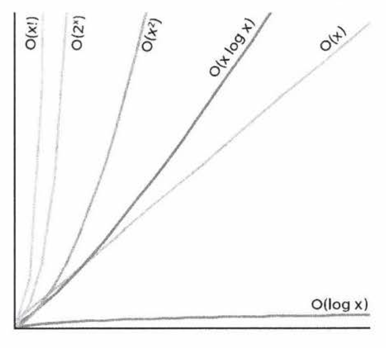
Variables used in Big O notation denote the sizes of inputs to algorithms. The following examples of common complexities and their Big O notations are ordered from fastest to slowest.

Constant - O(1)

Given an input array A = [1,2,3,4,5] write a function that returns the first element of the array. The solution will run in constant time, i.e., O(1).

def first_elem(A):
  return A[0]

Many people confuse O(1) with “doing only one thing”, but they are not the same thing. In the above example, if our function returned the first three elements of the array, it would still be O(1), because big O notation measures the increase rate of our computation time given the input size.

Logarithmic - O(log(n))

log₂N = k -> 2^k = N

When you see a problem where the number of elements in the problem space gets halved each time, that will likely be a O(log N) runtime.

This halving is why finding an element in a balanced binary search tree is O(log N). With each comparison, we go either left or right. Half the nodes are on each side, so we cut the problem space in half each time.

Linear - O(n)

You are given an array A = [1,2,3,4,5] and you have to write a function that returns the squares of the array A. To solve this, we need to create an array B that will contain the squares of the input. We start at the element A[0] and square it and store it in B[0], next we square A[1] and store it in B[1], all the way to the last element of input array A. In other words, we need to iterate all the input array an calculate, i.e., the time that our algorithm will take is proportional to the number of elements N in the input array. Hence, our algorithm is O(N).

Log-Linear - O(nlog(n))

Quadratic - O(n²)

If we want to generate all different pairs that we can form using an input array A = [1,2,3,4,5], for each of the elements, we need to iterate the rest of the array, i.e., O(n²).

Polinomial - O(n^c)

Exponential - O(cⁿ)

Recursive calls: O(branches^depth)

If there are two branches per recursive call, and we go as deep as N, therefore, the runtime is O(2^N).

Generally speaking, when you see an algorithm with multiple recursive calls, you look at exponential runtime.

Memoization is a technique used to optimize exponential time recursive algorithms.

Factorial - O(n!)

Important concepts

• Drop the constants

• Drop the non-dominant terms

• Multi-part algorithms: add vs multiply

Suppose you have an algorithm that has two steps. When do you multiply the runtimes and when do you add them?

Add the runtimes: O(A + B)

for(int a: arrA) {
  print(a);
}

for(int b: arrB) {
  print(b);
}

In this example, we do A chunks of work, then B chunks of work. Therefore, the total amount of work is O(A + B).

Multiply the runtimes: O(A * B)

for(int a: arrA) {
  for(int b: arrB) {
    print(a + "," + b);
  }
}

In this example, we do B chunks of work for each element in A. Therefore, the total amount of work is O(A * B).

• In the context of coding interviews, Big O notation is usually understood to describe the worst-case complexity of an algorithm

Amortization

The operation takes T(n) amortized time if any k operations take <= k * T(n) time.

(Particular kind of averaging. Averaging over the sequence of operations.)

Some individual operations are expensive, but most operations are cheap, so you average all operations.

Not as good as constant time but almost as good.

Examples:

• Insert at the end of a vector (dynamic array)
• Hash table look-up

Sources:

• Big Oh Cheat Sheet
• mycodeschool
• CTCI - chapter VI
• Time & Space Complexity - Big O Notation